Recently, a friend of mine embarked on an excursion through the mountains of Northern Italy, capturing the essence of wilderness through a snapshot of wolf paw imprints in the snow.

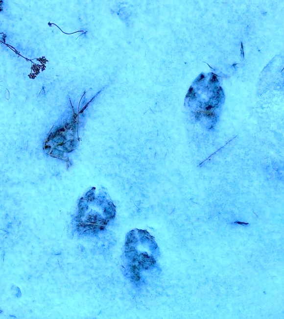
As I examined the photo, an echo from the past reverberated—a conversation with an old man fifteen years ago, who mused with a knowing smile: “Where wolves roam, something to hunt surely have passed”.

Ecology unfolds like a compelling saga, a tale of interconnectedness where predators and prey perform a dance, shaping the oscillating balance of ecosystems. The presence of wolves signals more than their mere existence; it reveals the interplay within Nature’s theater.

Predator-prey interactions orchestrate population dynamics, influencing not just the species involved but also the entire ecosystem. This dance of life embodies the essence of coexistence—predators relying on prey for sustenance, while the prey’s survival tactics evolve under the persistent pressure of predation.

This dynamic balance was elegantly captured in the early 1900 by the scientists Alfred Lotka (1925) and Vito Volterra (1926), at least in its very fundamental aspects. The model named after them, the “Lotka-Volterra model”, is an effective mathematical representation that depict the intertwined nature of predator and prey populations.

Based on a couple of differential equations, the model considers two interacting species: predators (e.g., wolves) and prey (e.g., deer, or rabbits). The assumptions of the model are: I) there is an exponential population growth, like if they were in absence of any limiting factors; II) the predator can only predate on the prey designated in the model – thus other food sources are not considered; III) no competition effect or density-dependent negative factors are taken into account.

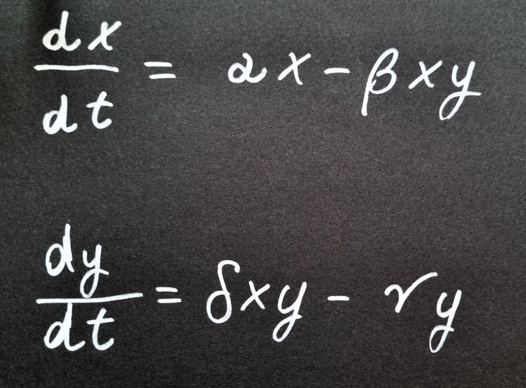
So, let’s represent the prey population, namely the number of individuals in the prey population, as the x , and let ‘y’ represent the predator population. According to Lotka and Volterra, the rate of change of the prey population (x) over time is influenced by the number of prey individuals born at each time unit (look at the first addendum, αx), and by the number of individuals prelevated from the population due to predation exerted by the interacting population of predators (indeed the second addendum has a coefficient β that is multiplicated times x and y). Similarly, the rate of change of the predator population depends on two primary factors: firstly, the number of predators sustained by “successful” interactions with the prey population, and secondly, the number of predators lost from the population due to death caused by various factors (with γ denoting something similar to the intensity of these factors).

You can start plugging some placeholder values to explore what the maths says, but I believe that considering changes instead of absolute values provides a clearer insight into population dynamics. Take a closer look at the second equation, and try to convert it into images of, say, wolves and rabbits: now it is easy to grasp the idea that an increase in prey population leads to a subsequent increase in the predator population as a result of the product xy. This occurs when there is a lot of meaty food available: in our example, more rabbits to eat means more energy for wolves, providing resources to survive and eventually reproduce by giving birth to wolf cubs.

And wolves in happy families eat a lot, so as the wolf population grows, more attacks on the rabbit population occur.

This is exactly what the first equation suggests: as the predator population increases, more predation takes place. Also in this case, try to visualize in the first equation, leading to a faster decline in the rabbit population… perhaps as the cubs learn to hunt.

As you may notice, these relationships between predator and prey populations may result in cyclic or oscillating behaviors. When the prey population increases, the predator population also increases, after a certain time-lag, due to the abundance of food. However, as the predator population grows, it exerts more pressure on the prey, soon causing the prey population to decline. As a result, the predator population eventually decreases due to a lack of food, allowing the prey population to recover and restart the cycle.

An equilibrium can still occur, though. Let’s study the system of equations by setting the rate of changes in population to zero, simulating that the number of individuals in the population remains constant, hence x′(t) and y′(t) are equal to zero.

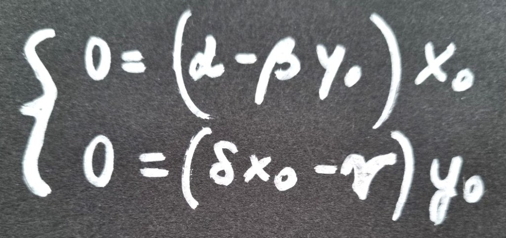
By solving this system of equations, we find two solutions for the pair (x0​,, y0), corresponding to two equilibrium points: (0,0) or (δ/γ,α/β). The first corresponds to the extinction of both species: if both populations have 0 individuals, they will maintain this number at every subsequent moment. No rabbits, no wolves – and no bunnies, nor cubs.

The second equilibrium point, however, represents the case where predators consume, for each time unit, a number of prey that is exactly equal to the number of prey being born. This number of prey corresponds precisely to the critical threshold of food that keeps the predator population stable.

However, this model, though foundational, encounters limitations when applied to real-world scenarios. Nature, with its complexities, defies a one-size-fits-all approach. Factors like environmental and habitat changes, multiple prey species, and additional interactions among species challenge the model’s accuracy.

In response to these limitations, contemporary ecologists have developed more nuanced population models. These newer models consider a broader array of factors, such as habitat variation, species interdependence, and stochastic events, offering a more comprehensive understanding of population dynamics within ecosystems.

Yet, amidst these sophisticated models and scientific endeavors, it’s crucial to acknowledge the wisdom harbored by local communities intimately connected to the land. Their deep-rooted knowledge often mirrors ecological truths: the adage shared by the old man I met is emblematic of the indigenous wisdom.

But this is another story I will tell you in another post.

In the meanwhile, predators and preys will continue their age-old dance, a rhythm as ancient as time itself, teaching us profound lessons in resilience, adaptability, and the interconnectedness of life.